 Roberto
1. Why the Direct Analysis Method (DAM)?
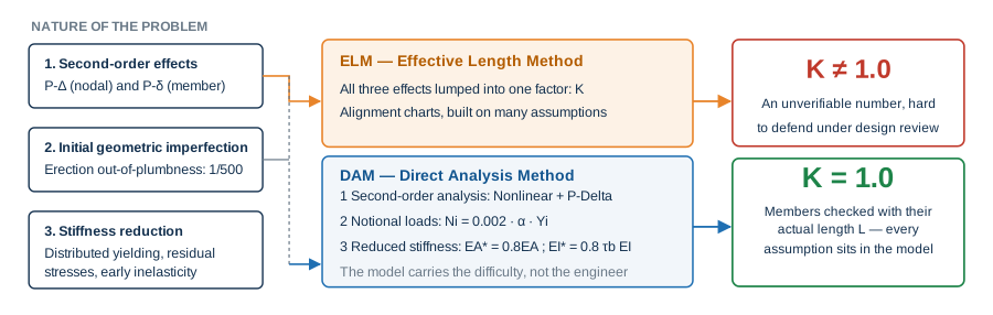
The strength of a steel column in a steel framing system does not depend on its section alone — it also depends on the flexibility of the whole system. AISC 360 requires stability to account for three factors at once:
- Second-order effects: P-Δ (joint displacement) and P-δ (flexural deformation within the member);
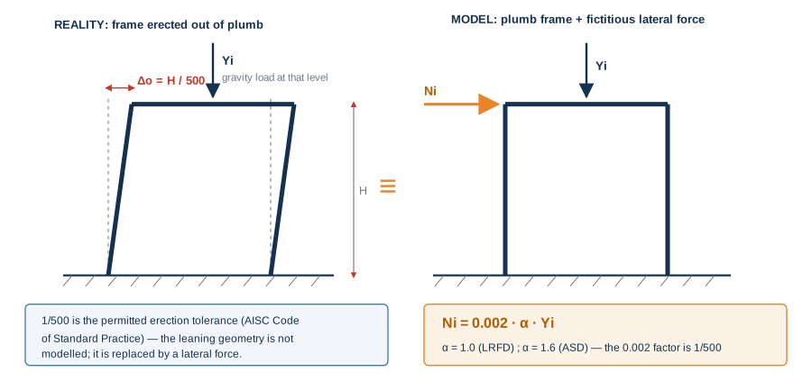
- Initial geometric imperfections: erection out-of-plumb, normally taken as 1/500;
- Stiffness reduction from partial yielding and residual stresses.
The Effective Length Method (ELM) compresses all three into a single number — the effective length factor K — then asks the engineer to read an alignment chart built on numerous assumptions and boundary conditions. K takes time to compute and keeps changing throughout the design. Eccentrically braced frames, equipment support columns, multi-level pipe racks, steel columns on RC pedestals… all demand considerable effort to compute and to keep under control.
DAM inverts that logic: the model carries the hard part — through second-order analysis, notional loads and stiffness reduction — and members are checked with K = 1.0, using their actual length. For steel structures this is not merely the “modern” choice; it is the only one that protects the engineer when K has to be justified.
The three mandatory DAM conditions
| Clause | Requirement | Formula | Where to set it in SAP2000 |
|---|---|---|---|
| C2.1 | Second-order analysis (P-Δ and P-δ) | — | Nonlinear Static + P-Delta; divide frame |
| C2.2b | Notional load at each level | Ni = 0.002·α·Yi, α = 1.0 (LRFD) / 1.6 (ASD) | Load Pattern type NOTIONAL |
| C2.3 | Stiffness reduction | EA* = 0.8EA; EI* = 0.8·τb·EI | Frame Property Modifiers |
| C3 | Check members with K = 1.0 | Lc = L | Steel Frame Design Overwrites |
where τb = 1.0 when αPr/Py ≤ 0.5, and τb = 4(αPr/Py)[1 − αPr/Py] when αPr/Py > 0.5.
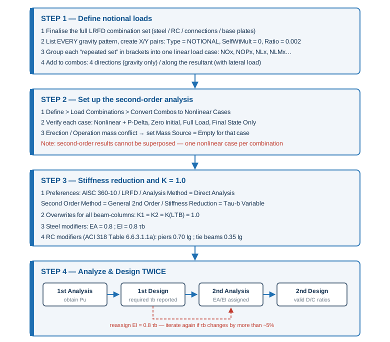
2. STEP 1 — Defining the notional loads
A notional load is an equivalent lateral force standing in for a 1/500 out-of-plumb column: 0.002 times the gravity load at the level considered, distributed the same way that gravity load is distributed (§C2.2b(3)).
2.1 The order of definition
(a) Define the LRFD combinations first. Notional loads are required within the combinations: each combination carries its own gravity mix, so the full combo list must exist before you start.
(b) List every load pattern that is a “gravity load” — not just dead load. In industrial structures this list is longer than expected: self weight (BL), superimposed dead (DL), equipment empty (EE), operating (EOL), hydrotest water (ETL), floor live (LL), monorail (LLM)… Miss one pattern and you are missing its notional load.
(c) Create a notional load pattern pair for every gravity load in the X and Y directions (a compact naming convention: xDL/yDL, xEE/yEE…):
Define > Load Patterns
  Load Pattern Name : xDL
  Type              : NOTIONAL
  Self Weight Mult. : 0
  Auto Lateral Load : Auto
  → Modify Lateral Load Pattern...
       Base Load Pattern : DL
       Load Ratio        : 2.000E-03
Direction : Global X / Global Y2.2 The “repeated set” technique — 40 patterns down to 8 load cases
Adding notional patterns straight into each combination means one factor line per pattern per combination. Instead, look at the bracket structure of the combination:
1.2·(D + Dsup + EE + EOL) + 1.6·(L + Lmono)
      └──── repeated set ────┘   └─ repeated set ─┘
Each bracketed set reappears in many combinations with the same factor. So collapse the notional loads of the whole set into a single linear load case:
| Repeated gravity set | Notional load case (X) | Load case content |
|---|---|---|
| D + Dsup + EE | NOx | xD + xDsup + xEE |
| D + Dsup + EE + EOL | NOPx | xD + xDsup + xEE + xEOL |
| L | NLx | xL |
| L + Lmono | NLMx | xL + xLmono |
| L + 1.4·Lmono | NLM2x | xL + 1.4·xLmono |
Define each load case as Static / Linear / Zero Initial Conditions, combining the notional patterns with scale factors matching the ratios inside the bracket. The combination then needs 2 extra lines instead of 20:
Combo: 1.2·(D+Dsup+EE+EOL) + 1.6·(L+Lmono) + 1.2·NOPx + 1.6·NLMx2.3 Direction of the notional load
§C2.2b(3): the notional load must act in the direction that increases the destabilising effect of the combination being considered.
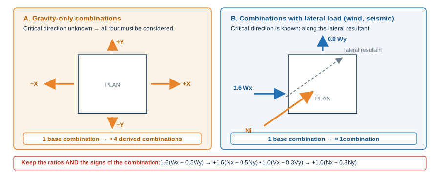
| Combination type | Notional direction | Derived combinations |
|---|---|---|
| Gravity only | All four: +X, −X, +Y, −Y (the governing direction is unknown) | × 4 |
| With lateral load (W, E) | Along the resultant lateral force of that combination | × 1 |
For a wind combination 1.6·(WX + 0.5·WY) the notional loads follow the same ratio → +1.6·(Nx + 0.5·Ny). For a seismic combination 1.0·(VX − 0.3·VY) → +1.0·(Nx − 0.3·Ny).
3. STEP 2 — Setting up the second-order analysis
The important rule: second-order analysis does NOT superpose. You cannot run P-Delta on each pattern and add the results linearly in a combination. Every design combination must be its own independent nonlinear static case, carrying the full factored load.
3.1 Converting combinations into nonlinear cases
Define > Load Combinations > Convert Combos to Nonlinear Cases...
  → select every LRFD combination → OK
  (SAP2000 creates LCxxxx-NL, and rewrites combo LCxxxx as: 1.0 × LCxxxx-NL)
After converting, open two or three cases at random and check them:
| Field | Correct value |
|---|---|
| Load Case Type / Analysis Type | Static / Nonlinear |
| Geometric Nonlinearity | P-Delta |
| Initial Conditions | Zero Initial Conditions |
| Loads Applied | every pattern with the combination factors (0.9, 1.2, 1.6…) |
| Load Application | Full Load |
| Results Saved | Final State Only |
3.2 A note on mass source (erection vs. operation)
A common error on an analysis model:
Load Case LC1009-NL reset not to run.
Conflicting mass sources for included Load Pattern VX(E).
The cause: a nonlinear case contains an equivalent-static seismic pattern tied to the “Erection” mass source while the case itself uses “Operation” (or the reverse). The fix: mass plays no part in a static nonlinear case → set Mass Source = Empty for it. The seismic force is already a pre-computed static force; no mass is needed.
4. STEP 3 — Stiffness reduction and K = 1.0
4.1 Design preferences
Design > Steel Frame Design > View/Revise Preferences
  Design Code                : AISC 360-10
  Design Provision           : LRFD
  Multi-Response Case Design : Envelopes
  Analysis Method            : Direct Analysis        ← essential
  Second Order Method        : General 2nd Order      ← essential
  Stiffness Reduction Method : Tau-b Variable  (or Tau-b Fixed = 1.0, see Tip 6)
4.2 Overwrites: forcing K = 1.0
Design > Steel Frame Design > View/Revise Overwrites  (select all beam-columns)
  Effective Length Factor K1 Major / K1 Minor : 1.0
  Effective Length Factor K2 Major / K2 Minor : 1.0
Effective Length Factor K (LTB) : 1.0KLTB = 1.0 is the conservative choice per AISC 360-10 Commentary E4 (the program already defaults to 1.0 for beams, but state it explicitly so the calculation record is transparent).
4.3 Property modifiers for steel members
Assign > Frame > Property Modifiers for every member participating in the lateral system:
| Modifier | Value | Note |
|---|---|---|
| Cross-section (axial) area | 0.8 | Mainly affects braces and truss members |
| Moment of inertia about axes 2 & 3 | 0.8 × τb | τb depends on Pu → iteration required |
| Torsional constant, shear area | 1.0 | AISC requires no reduction |
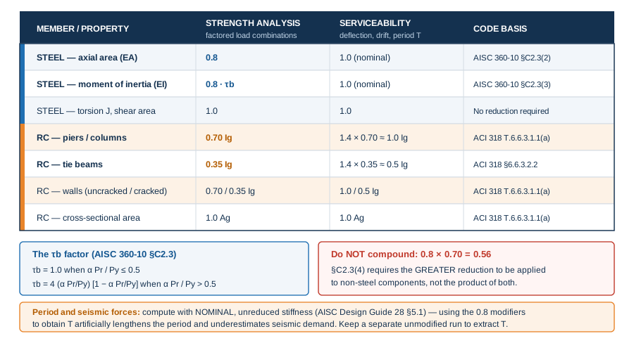
Note: these reductions are for strength analysis. Do not use them for serviceability deflection checks, and do not use them to compute vibration periods (§4.4).
4.4 RC pedestals and tie beams in the same model
AISC 360-10 §C2.3(4): where members of a material other than steel contribute to system stability and the governing code for that material requires a larger reduction, the larger reduction applies. Per ACI 318-14 Table 6.6.3.1.1(a) (unchanged in 318-19/318-25):
| Member | Strength (factored) | Immediate lateral deflection — §6.6.3.2.2 (1.4·I, ≤ Ig) |
|---|---|---|
| RC pedestal / column | 0.70·Ig | 1.4 × 0.70 ≈ 1.0·Ig |
| RC tie beam | 0.35·Ig | 1.4 × 0.35 ≈ 0.5·Ig |
| Wall (cracked / uncracked) | 0.35 / 0.70·Ig | as above |
| Area | 1.0·Ag | 1.0·Ag |
Set them at: Define > Section Properties > Frame Sections > Modify/Show Property > Set Modifiers
5. STEP 4 — Analyse & design twice
τb depends on Pu, and Pu depends on the stiffness of the model → an iterative problem:
   [1] Run Analysis  (with no modifiers, or estimated ones)
            ↓  read Pu for each member
   [2] Run Steel Design  → the program reports the required τb
            ↓  re-assign EA = 0.8 ; EI = 0.8·τb
   [3] Run Analysis, 2nd pass   ← the real analysis, on reduced stiffness
            ↓
   [4] Run Steel Design, 2nd pass  → D/C ratios valid for issue
If the second pass changes any section or shifts τb appreciably (> ~5%), run one more cycle.
6. Seven things to know before pressing Run
(1) No intermediate node → the P-δ effect is lost entirely. The frame element P-Delta formulation only captures P-Δ between its two end nodes. Dividing the frame is mandatory:
Assign > Frame > Automatic Frame Mesh...
  ◉ Auto Mesh Frame
  ☑ at Intermediate Joints
  ☑ Minimum Number of Segments : 2   (2–4 recommended for heavily loaded columns)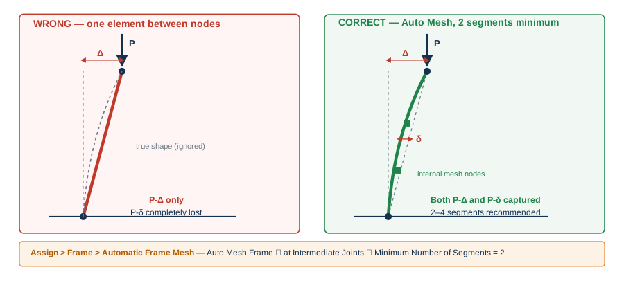
Automatic Frame Mesh is enough: auto mesh subdivides the element internally for analysis only; the design object, its unbraced lengths and its design section stay intact.
(2) K = 1.0 does not mean the length is right. DAM frees you from K, not from L. The Unbraced Length Ratio (Major / Minor / LTB) remains the engineer's responsibility: does the purlin actually brace the compression flange? At what level does the column get a lateral strut? This is the largest source of error in any steel problem, DAM or not.
(3) SAP2000 does not compute B2. The “amplified first order” method needs B1 and B2; SAP2000 currently always takes B2 = 1.0. So choose only Second Order Method = General 2nd Order. If someone selects “Amplified 1st Order” in the preferences, the results will omit the global second-order effect entirely.
(4) Vibration periods must come from nominal stiffness. AISC Design Guide 28 §5.1: seismic forces and the period T are computed on unreduced sections. Using the 0.8 modifier to find T lengthens the period artificially → seismic forces are underestimated. In practice: keep a separate model or run (or a separate modifier set) with no reduction to extract T and the seismic forces, and only then apply the modifiers for the strength analysis.
(5) Serviceability deflection ≠ reduced stiffness. Beam deflection checks, service lateral drift and camber calculations all use nominal stiffness (for RC: 1.4·I, ≤ Ig).
(6) A nonlinear case will not converge. Do not reach for more steps or a looser tolerance. Divergence in P-Delta is almost always a recurring underlying problem. Check:
(a) is the system genuinely unstable — run Modal, look for a mode with an implausibly long period or a nonsensical local shape, and find the member with a missing connection or a wrong release;
(b) is the system too “flexible” — if Δ2nd/Δ1st > 1.7, the structural scheme itself needs more bracing, not more iterations.
(7) Design combinations do not update themselves. After Convert Combos to Nonlinear Cases, open Design > Steel Frame Design > Select Design Combos and confirm the program is checking the converted combinations, not a default set it generated on its own.
7. A field guide for the structural engineer
The fast, sensible check: pick one governing member, Design > Steel Frame Design > Display Design Info → Steel Stress Check Data. Then compare:
| Line in the output | Value that must appear |
|---|---|
| Design code | AISC 360-10 |
| Provision | LRFD |
| Analysis | Direct Analysis |
| 2nd Order | General 2nd Order |
| Reduction | Tau-b Variable (or Tau-b Fixed) |
Tau_b | 1.0 if αPr/Py ≤ 0.5 |
EA factor / EI factor | 0.800 / 0.800·τb |
K1, K2 (major & minor) | 1.000 |
Kltb | 1.000 |
Length, Lltb | the real unbraced length |
Checklist before issuing the design
- Every gravity load pattern listed, each with its matching X/Y notional pair
Self Weight Multiplier= 0 on every notional pattern- ΣFX(notional) = 0.002 (or 0.003) × ΣFZ(source pattern) — verified through Base Reactions
- Gravity-only combinations: all four notional directions; lateral combinations: notional along the resultant, with the correct sign
- Every design combination is Nonlinear Static + P-Delta; the erection/operation mass source conflict is resolved
- Auto Mesh Frame ≥ 2 segments on every compression member
- Modifiers: steel EA=0.8, EI=0.8τb; RC pedestals 0.70Ig, tie beams 0.35Ig
- K1 = K2 = KLTB = 1.0; unbraced lengths reviewed visually on the 3D model
- Period T and seismic forces taken from nominal stiffness
- Analyse → Design run twice (or the 0.003 + τb=1.0 route used)
- Δ2nd/Δ1st checked; if ≤ 1.7, recorded in the report to justify omitting notional loads from lateral combinations
- No warnings left in the analysis log; every case converged
8. Closing
DAM shifts the burden from computing the K factor to the honesty of the model. That is a favourable trade: K takes time to compute and keeps changing throughout the design, whereas a model can be checked line by line — through base reactions, through displacement ratios, through the Steel Stress Check Data output.
Three points to carry away:
(1) notional loads must cover every gravity load and act in the governing direction;
(2) each combination is its own P-Delta nonlinear case, and members must have intermediate nodes;
(3) K = 1.0 only means something once the analysis has run on reduced stiffness — prove it with the EA factor = 0.800 line in the output.
References
- AISC 360-10, Specification for Structural Steel Buildings, Chapter C & Commentary, American Institute of Steel Construction, Chicago, 2010.
- AISC Design Guide 28, Stability Design of Steel Buildings, §5.1.
- ACI 318-14, Building Code Requirements for Structural Concrete, §6.6.3.1.1 & §6.6.3.2.2.
- CSI, Practical How-To Guide Technical Note — AISC Direct Analysis Method, Computers and Structures, Inc., California.
- CSI, Steel Frame Design Manual — AISC 360-10 / IBC 2012 for SAP2000.
Part of the series “Structural design for industrial facilities” — Roberto Structural. The content is technical guidance; the engineer remains responsible for checking and adapting it to the conditions of each project and the requirements of the governing code.